An integrated map of structural variation in 2,504 human genomes(Summary)

2015, Nature, 2077 citation (69.504 impact factor)

https://www.nature.com/articles/nature15394

Abstract
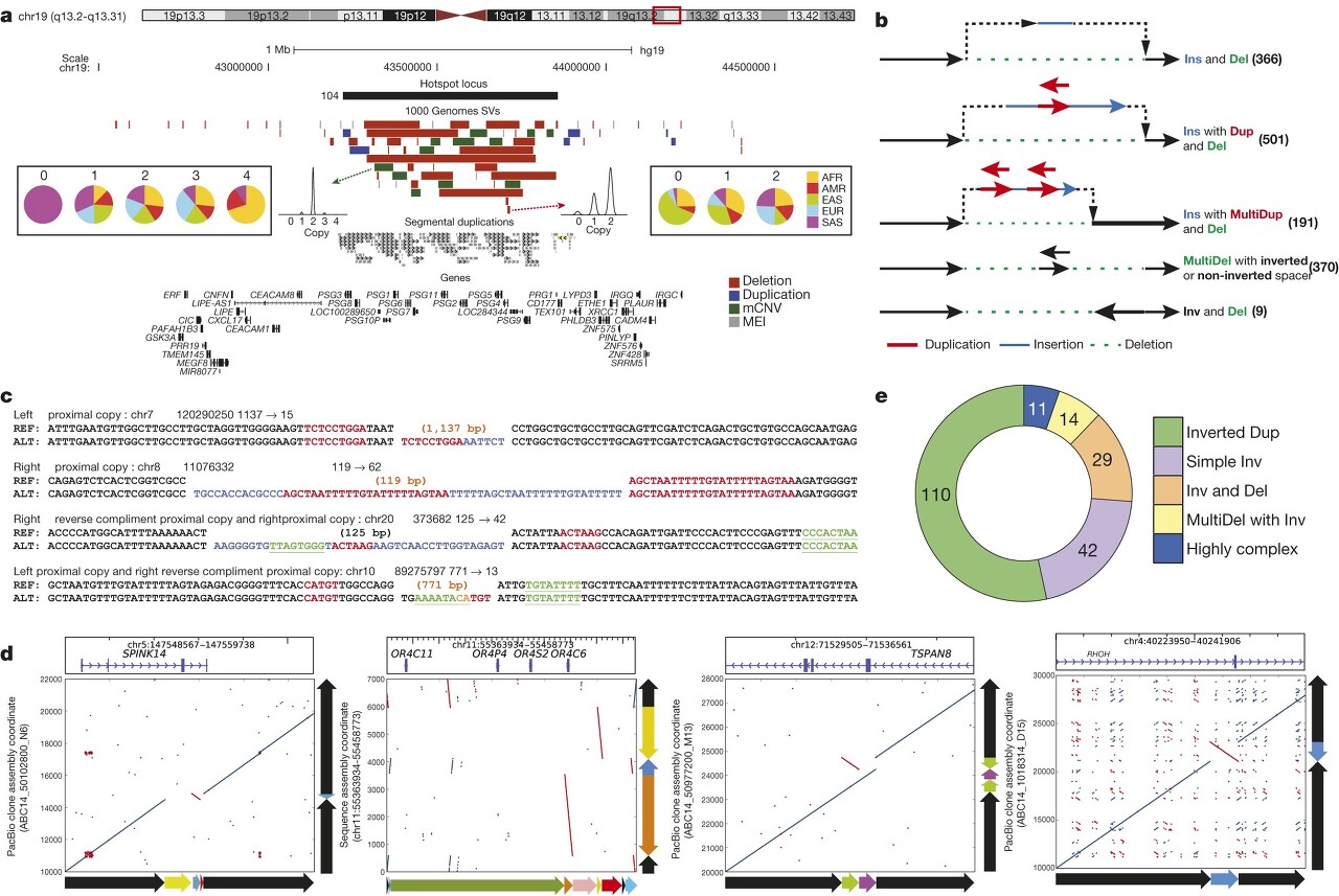
we describe an integrated set of eight structural variant classes comprising both balanced and unbalanced variants
균형있고 변이와 불균형한 변이를 비교하여 8 개의 SV 클래스를 정의
we constructed using short-read DNA sequencing data and statistically phased onto haplotype blocks in 26 human populations
26 인종에 대하여 short-read DNA seq 데이터를 사용했으며, SV를 추정하기위해 statistically phased onto haplotype blocks 기법을 사용했다.

 

Introduction

- 구조적 변이(Structural variants, SVs)는 개인의 인간 유전체 중 가장 다양한 염기쌍(base pairs, bp)을 차지하는 것

- 삭제(deletions), 삽입(insertions), 복제(duplications) 및 역전(inversions) 등을 포함

- 많은 연구에서는 SVs가 인지능력 장애부터 비만, 암 등과 관련된 표현형을 가지는 인간 건강과 관련이 있다고 밝힘

- 그러나 SV 구조가 복잡하며, 반복적인 영역에서 발생하여 식별의 어려움이 존재

- GWAS 분석으로도어려움이 존재

- Despite recent methodological and technological advances, efforts to perform discovery, genotyping, and statistical haplotype-block integration of all major SV classes have so far been lacking.

모든 주요 SV 클래스를 발견하고, 통계적인 헤플로타입 블록 통합을 수행에 부족했음

- 또한 소수의 샘플을 대상으로한 microarray 데이터 사용.

 

-The objective of the Structural Variation Analysis Group has been to discover and genotype major classes of SVs (defined as DNA variants ≥50 bp) in diverse populations and to generate a statistically phased reference panel with these SVs.

: 다양한 인구에서 주요한 SV 클래스(≥50 bp의 DNA 변이로 정의)를 발견하고 유형화하며, 이러한 SV들을 통계적으로 페어링된 참조 패널로 생성하는 것

 

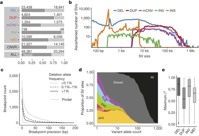
- Here we report an integrated map of 68,818 SVs in unrelated individuals with ancestry from 26 populations

본 연구에서는 26개 인구에서 기원한 관련 없는 개인들의 68,818개의 SV를 포함하는 통합 맵을 보고

 

Methods

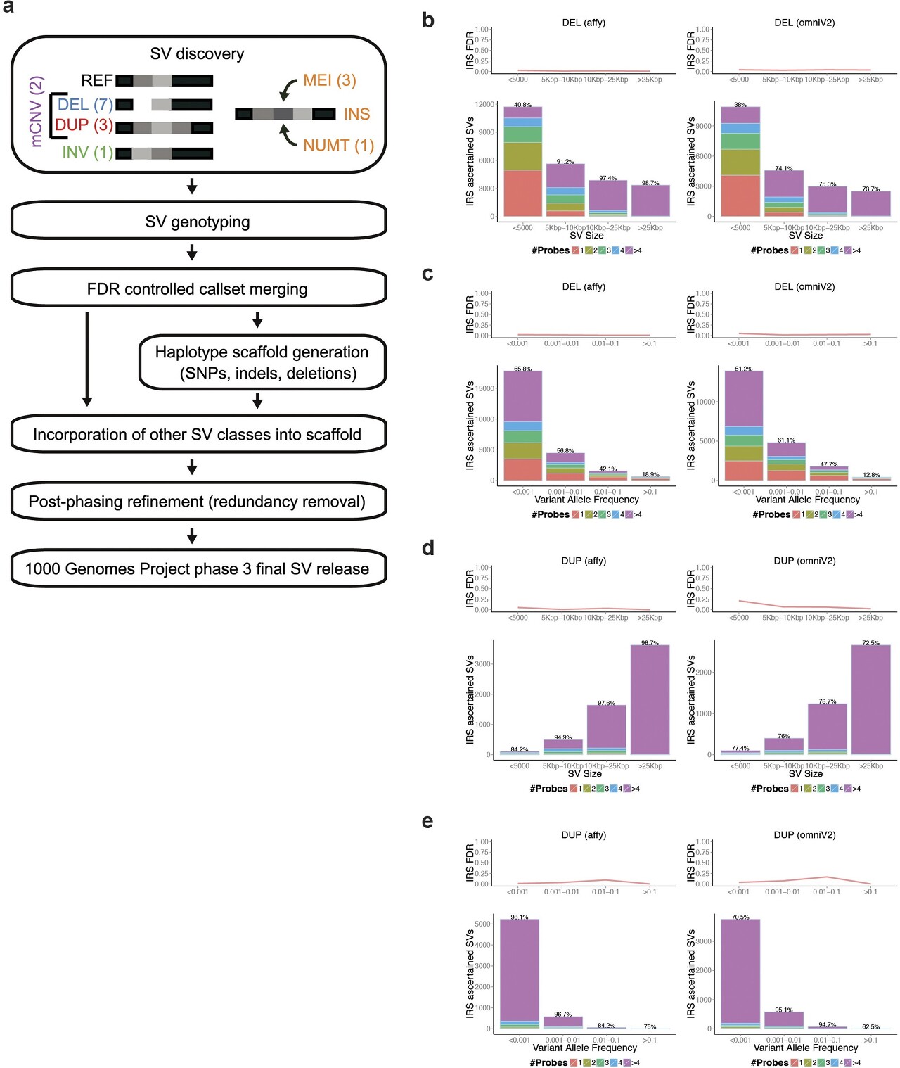
Construction of our phase 3 SV release

 

- We mapped Illumina WGS data (∼100 bp reads, mean 7.4-old coverage) from 2,504 individuals onto an amended version8 of the GRCh37 reference assembly using two independent mapping algorithms—BWA17 and mrsFAST18—and performed SV discovery and genotyping using an ensemble of nine different algorithms

: GRCh37 에 BWA, mrsFAST 을 이용해 Illumina WGS(약 100bp read, 7.4 coverage) 데이터를 어셈블

9개의 알고리즘의 앙상블로 SV 유형화

 

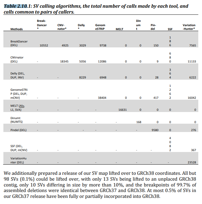
- We applied several orthogonal experimental platforms for SV set assessment, refinement and characterization (Supplementary Table 2) and to calculate the false discovery rate (FDR) for each SV class (Table 1)

9가지 다른 알고리즘의 앙상블을 사용하여 SV를 발견하였고, 이러한 결과의 FDR을 평가하기 위해 보조 실험 플랫폼을 적용. 이러한 보조 실험은 SV 세트의 평가, 개선 및 특성화를 위해 사용

-----------supple

BreakDancer, Delly, VariationHunter, CNVnator, Read-Depth(SSF), Genome STRiP, Pindel, MELT, Dinumt

두 방법 중 어느 두 방법에서도 공통 호출의 수가 표시됩니다.

- 다섯 가지 가장 구체적인 삭제 탐지 알고리즘(BreakDancer1, Delly3, CNVnator6, GenomeSTRiP14, VariationHunter5)로부터 호출된 사이트를GenomeSTRiP의 중복 제거 기능을 사용

a) Remove all duplicate calls using standard settings in Genome STRiP (50% site overlap and most discordant LOD score greater than zero).

b) Perform a second pass removing duplicate calls using criteria of site overlap greater than 50% and no discordant genotypes at a 95% confidence threshold.

c) Perform a third pass removing duplicate calls using criteria of 80% site overlap only.

The results of each merging pass are indicated in the three summary lines in Table 3.1 (Merge1, Merge2, Merged call set). FDR estimates (using the IRS method, Omni 2.5 array) ranged from 1% to 6.7% in the input call sets. The estimated FDR in the genotyped call set was 3.1%.

 

- Callset refinements facilitated through long-read sequencing enabled us to incorporate a number of additional SVs into our callset, including an additional 698 inversions and 9,132 small (<1 kbp) deletions, compared to the SV set released with the 1000 Genomes Project marker paper.

: long-read 시퀀싱을 통한 콜셋 개선을 통해 1000 Genomes 프로젝트 마커 논문16과 비교하여 추가적인 SV를 콜셋에 포함

 

- We merged individual callsets to construct our unified release (Table 1), comprising 42,279 biallelic deletions, 6,025 biallelic duplications, 2,929 mCNVs (multi allelic copynumber variants), 786 inversions, 168 nuclear mitochondrial insertions (NUMTs), and 16,631 mobile element insertions (MEIs, including 12,748, 3,048 and 835 insertions of Alu, L1 and SVA (SINE-R, VNTR and Alu composite) elements, respectively).

: short-read 9개 알고리즘 앙상블 결과와 long-read 1000 Genomes project marker 논문을 통합하여, 각 개인별 SV 통합한 결과

 

a, Approach used for constructing our SV release set. b, Intensity rank sum (IRS) validation results for deletions in different size bins. c, IRS validation results for deletions in variant allele frequency (VAF) bins. d, IRS results for duplications in different size bins. e, IRS validation results for duplications in VAF bins. Based on Affymetrix SNP6 array probes, the IRS FDR for all SV length and VAF bins was &le;5.4%, requiring at least 100 SVs per bin with an IRS assigned P-value.

 

a, &nbsp;Novelty based on overlap of our SV set with DGV 19 &nbsp;(upper panel, broken down by SV class), of collapsed CNVRs with earlier 1000 Genomes Project releases 6,8 &nbsp;(middle panel) and of our SV set with refs&nbsp; 6 ,&nbsp; 8 &nbsp;(bottom panel).&nbsp; b, &nbsp;Size distribution of ascertained SVs (bin width is uniform in log-scale). DEL, biallelic deletion, DUP, biallelic duplication, INV, inversion, INS, non-reference insertion (including MEIs and NUMTs).&nbsp; c, &nbsp;Breakpoint precision of assembled deletions stratified by VAF (split-read caller Pindel 23 &nbsp;shown separately).&nbsp; d, &nbsp;SV allele sharing across continental groups.&nbsp; e, &nbsp;LD properties of biallelic SV classes.

SV clustering and complexity

- We identified 3,163 regions where SVs seemed to cluster (>2 SVs mapping within 500 bp; Supplementary Table 11).

- To reduce redundancy caused by multiple overlapping calls per sample, we calculated distinct CNVRs per cluster by merging calls per sample and haplotype and then counting the distinct CNVRs produced across samples (average 6.4 ± 7.2 CNVRs per cluster).

 

CNVR (Copy Number Variable Regions)를 클러스터링하기 위해 다음과 같은 방법을 사용했습니다:

1. SV 데이터에서 CNVR이 군집화된 지역 3,163개 식별
   이는 500 bp 내에서 2개 이상의 SV가 매핑된 지역을 의미.
2. 이렇게 찾은 군집당 평균 6.4개의 고유한 CNVR 있는 것으로 확인
3. 각 군집(cluster)당 distinct CNVR 수, samples 수를 조사

이러한 접근 방식을 통해 CNVR 군집화를 수행하여 복잡성과 패턴을 파악할 수 있었습니다.

a, &nbsp; PSG &nbsp;locus with clustered SVs. Population copy-number state histograms are shown for two example SVs.&nbsp; b, &nbsp;Schemes depicting assembled complex deletions.&nbsp; c, &nbsp;Smaller-scale complex deletions identified with Pindel 23 . Flanking sequences are shown for reference (REF) and alternate (ALT) alleles, further to insertions at the breakpoints. Proximal stretches matching the insertion are labelled in red (forward) and green (reverse complement). Blue, insertions lacking nearby matches.&nbsp; d, &nbsp;Alignment dot plots depicting inversions (inverted sequences are in red within each dot plot). Adjacent schemes depict allelic structures for REF and ALT.&nbsp; e, &nbsp;Inversion complexity summarized.